Chapter 8 Diffusion Models 扩散模型

这个模型很有意思，我会尝试使用PyTorch实现。

介绍

扩散模型是过去十年中引入的最具影响力和影响力的图像生成生成建模技术之一。扩散这个名字的灵感来自于热力学扩散特性

突破性的扩散模型论文于 2020 年夏天发表。该论文揭示了扩散模型和基于分数的生成模型之间的深层联系，作者训练了一个扩散模型，可以在多个数据集胜过竞争对手 GAN，称为去噪扩散概率模型 (DDPM)

扩散电视

我们再次从一个小故事开始。

💡 您站在一家出售电视机的电子商店里。这里有数百台相同的电视机按顺序连接在一起，一直延伸到商店的后面。更奇怪的是，最前面的几台电视机似乎只显示随机的静态噪声。 店主解释说，这是新的DiffuseTV型号。在制造过程中，DiffuseTV接触了数千张以前的电视节目的图像，但是这些图像都被逐渐加入了随机的静态噪声，直到它们与纯随机噪声无法区分。然后，电视机被设计成以小步骤消除随机噪声，尝试预测在加入噪声之前图像是什么样子的。 可以看到，当走进商店时，每台电视机上的图像确实比上一台稍微清晰一些。 最终到达了一长排电视机的尽头，在那里您以看到最后一台电视机上的完美画面。 观众不是选择要观看的频道，而是选择一个随机的初始静态配置。每个配置都会导致不同的输出图像，而且在某些型号中甚至可以由您选择输入的文本提示来指导。与只有有限范围的频道可供观看的普通电视机不同，DiffuseTV给观众无限的选择和自由，可以生成他们想要出现在屏幕上的任何东西！

Denoising Diffusion Models (DDM)

我们尝试使用系列小步骤来给图像“降噪”。最终我们能从一个纯粹的随机噪音开始，逐步降噪到一个看起来是训练集中的数。

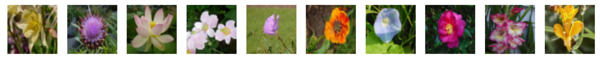
The Flowers Dataset

Flowers Dataset中包含8000张上色的花朵图片。每张图片为$64\times64$的尺寸。

代码实现

Keras的代码中有几处细节：

train_data = utils.image_dataset_from_directory(
    TRAIN_DATA_PATH,
    labels=None,
    image_size=(IMAGE_SIZE, IMAGE_SIZE),
    batch_size=None,
    shuffle=True,
    seed=42,
    interpolation="bilinear",
)
def preprocess(img):
    img = tf.cast(img, "float32") / 255.0
    return img
train = train_data.map(lambda x: preprocess(x))
train = train.repeat(DATASET_REPETITIONS)
train = train.batch(BATCH_SIZE, drop_remainder=True)

1. 在使用image_dataset_from_directory 的过程中没有指定batch，而是在之后使用train.batch(BATCH_SIZE, drop_remainder=True) 指定，这是为了丢弃最终不足一个批次的数据。我们可以指定PyTorch的DataLoader的drop_last=True来实现
2. train = train.repeat(DATASET_REPETITIONS) 将数据重复了五边。我们可以简单的自定义一个数据集类来实现。

class FLowerDataset(Dataset):
    def __init__(self, data_dir, transform, repetitions):
        self.data = datasets.ImageFolder(data_dir, transform=transform)
        self.repetitions = repetitions

    def __getitem__(self, index):
        orig_index = index % len(self.data)
        img, label = self.data[orig_index]
        return img, label

    def __len__(self):
        return len(self.data) * self.repetitions

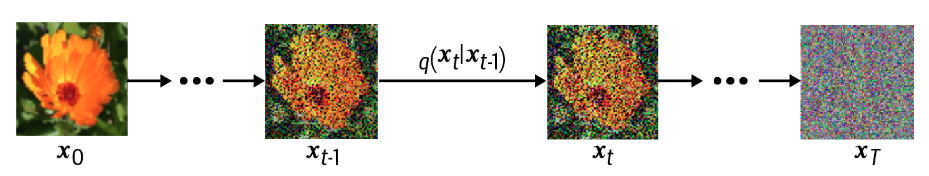
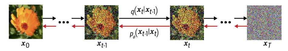
前向扩散过程

我们有一个图像 ，我们希望通过大量步骤逐渐损坏它，以便最终它与标准高斯噪声无法区分。

前向扩散原理

我们可以定义一个函数 $q$，将少量方差为 $β_t$ 的高斯噪声添加到图像。

由此，向前扩散的过程可以表示为：

$$\mathbf{x}_t=\sqrt{1-\beta_t} \mathbf{x}_{t-1}+\sqrt{\beta_t} \epsilon_{t-1}$$

其中，$\epsilon{t-1}$是一个标准正太分布。之所以同时对$x{t-1}$进行缩放是希望在整个过程中图像的方差保持。$\operatorname{Var}(X+Y)=\operatorname{Var}(X)+\operatorname{Var}(Y)$。

由此，我们可以定义q

$$q\left(\mathbf{x}_t \mid \mathbf{x}_{t-1}\right)=\mathscr{N}\left(\mathbf{x}_t ; \sqrt{1-\beta_t} \mathbf{x}_{t-1}, \beta_t \mathbf{I}\right) = LG\left(\mathbf{x}_t ; \sqrt{1-\beta_t} \mathbf{x}_{t-1}, \sqrt\beta_t \mathbf{I}\right)$$

重参数化技巧 Reparameterization Trick

相比于一个迭代的函数，我们更希望有一个函数，可以直接从图像$x_0$跳转到$x_t$。这一点我们通过重参数化技巧实现。

原理十分简单，我们使用$\alphat=1-\beta_t$和$\bar{\alpha}_t=\prod{i=1}^t \alpha_i$。

$$\begin{aligned}\mathbf{x}_t & =\sqrt{\alpha_t} \mathbf{x}_{t-1}+\sqrt{1-\alpha_t} \epsilon_{t-1} \\& =\sqrt{\alpha_t \alpha_{t-1}} \mathbf{x}_{t-2}+\sqrt{1-\alpha_t \alpha_{t-1}} \epsilon \\& =\cdots \\& =\sqrt{\bar{\alpha}_t} \mathbf{x}_0+\sqrt{1-\bar{\alpha}_t} \epsilon\end{aligned}$$

由此得到函数q

$$q\left(\mathbf{x}_t \mid \mathbf{x}_0\right)=\mathscr{N}\left(\mathbf{x}_t ; \sqrt{\bar{\alpha}_t} \mathbf{x}_0,\left(1-\bar{\alpha}_t\right) \mathbf{I}\right)$$

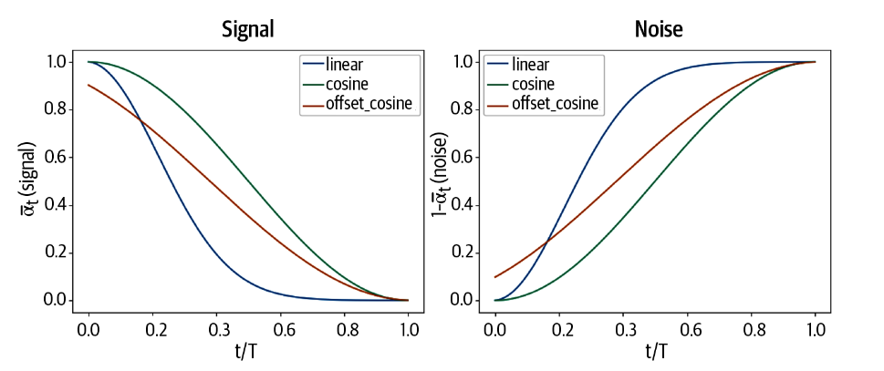
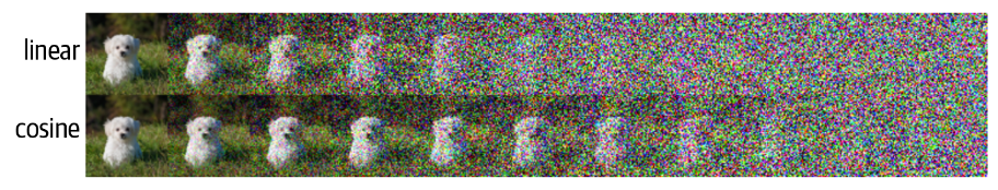
扩散方案

$\beta_t$可以随时间变化，原论文中，$\beta_t$被要求逐渐增大。即我们使用了线性的扩散方案。除此之外，原书还描述了cosine and offset cosine diffusion schedules。

通过这些方案，图像会逐渐接近于无法区分的标准高斯噪音。

简单的修改原书的Keras的代码，可以得到PyTorch的代码，如下。

def linear_diffusion_schedule(diffusion_times):
    min_rate = 0.0001
    max_rate = 0.02
    betas = min_rate + diffusion_times * (max_rate - min_rate)
    alphas = 1 - betas
    alpha_bars = torch.cumprod(alphas, dim=0)
    signal_rates = torch.sqrt(alpha_bars)
    noise_rates = torch.sqrt(1 - alpha_bars)
    return noise_rates, signal_rates
def cosine_diffusion_schedule(diffusion_times):
    signal_rates = torch.cos(diffusion_times * torch.pi / 2)
    noise_rates = torch.sin(diffusion_times * torch.pi / 2)
    return noise_rates, signal_rates
def offset_cosine_diffusion_schedule(diffusion_times):
    min_signal_rate = 0.02
    max_signal_rate = 0.95
    start_angle = torch.acos(torch.tensor(max_signal_rate))
    end_angle = torch.acos(torch.tensor(min_signal_rate))
    diffusion_angles = start_angle + diffusion_times * (end_angle - start_angle)
    signal_rates = torch.cos(diffusion_angles)
    noise_rates = torch.sin(diffusion_angles)
    return noise_rates, signal_rates

反向扩散过程

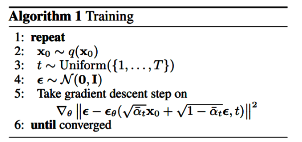
我们希望构建一个神经网络来消除噪音，来近似一个函数$P_\theta$。

这看起来与VAE很相似。他们之间的区别在于，在VAE中将模型转化为噪音也是学习的，而在diffusion中这是参数化的。因此应用类似于VAE的损失函数是有意义的。我们对图像$x_0$采样，并经过$t$步操作添加噪音。我们将这个添加噪音之后的图像和噪音率$\bar{\alpha}_t$提供给神经网络，并要求神经网络预测噪音$\epsilon$，并计算预测值和真值之间的均方差。

噪音消除过程

如上所属，经过训练的神经网络能够对噪音进行预测。下述代码中出现了两个模型，这两个模型在训练模型一部分描述。现在只需知道在训练过程和预测过程中，我们分别使用不同的模型即可。

def denoise(self, noisy_images, noise_rates, signal_rates, training):
        if training:
            network = self.network
            network.train()
            pred_noises = network([noisy_images,torch.pow(noise_rates,2)])
        else:
            network = self.ema_network
            with torch.no_grad():
                network.eval()
                pred_noises = network([noisy_images,torch.pow(noise_rates,2)])
        
        pred_images = (noisy_images - noise_rates * pred_noises) / signal_rates

        return pred_noises, pred_images

denoise 函数接受噪声图像、噪声率、信号率和一个表示是否在训练模式下的布尔值。如果在训练模式下，它会使用 self.network，否则会使用 self.ema_network。然后，它会计算预测的噪声和图像，并返回它们。

在模型对噪音进行预测后，我们进行噪音添加的逆向操作，按照噪音添加时的规则，逐步减去预测的噪音以获得原本的图像。

反向传播过程

不断重复这一过程，我们即可完成反向传播过程。在这一过程中，我们既使用了已经定义过的噪音去除过程不断地预测噪音和最初的图像，由进行正向传播中的噪音添加过程，来获得上一个图像。

def reverse_diffusion(self, initial_noise, diffusion_steps):
        # 获得图像的数量，盖为批次大小
        num_images = initial_noise.shape[0]
        # 获得每个扩散步数的大小
        step_size = 1.0 / diffusion_steps
        # 定义当前的图像为噪声
        current_images = initial_noise
        for step in range(diffusion_steps):
            # 扩散次数，因为是反向扩散，所以实际的应为1-当前扩散的次数/总次数
            diffusion_times = torch.ones((num_images,1,1,1))-step * step_size
            # 调用扩散方案，获得噪音率和信号率
            noise_rates, signal_rates = self.diffusion_schedule(diffusion_times)
            # 调用去噪函数，获得去噪后的噪声和图像
            pred_noises, pred_images = self.denoise(current_images, noise_rates, signal_rates, training=False)
            # 计算下一个扩散次数，和下一个噪音率和信号率
            next_diffusion_times = diffusion_times - step_size
            next_noise_rates, next_signal_rates = self.diffusion_schedule(next_diffusion_times)
            # 得到当前图像
            current_images = pred_images * next_signal_rates + pred_noises * next_noise_rates
        return pred_images

reverse_diffusion 函数接受初始噪声和扩散步骤的数量。它首先计算每个扩散步骤的大小，然后在每个步骤中，它会计算扩散时间、噪声率和信号率，然后调用 denoise 函数去噪，然后计算下一个扩散时间和下一个噪声率和信号率，最后更新当前的图像。这个过程会重复进行扩散步骤的数量次，最后返回预测的图像。

需要关注的是，只有最后一次循环得到的最初的图像在这一过程中被使用，此时上一个图像即为最初的图像。换句话说，我们会经过一系列小步骤得到图像而非一步到位。

图像生成

根据以上程序，我们可以使用模型生成图像。这里的denormalize 与图像最初的输入方式有关。

def generate(self, num_images, diffusion_steps, initial_noise=None):
        if initial_noise is None:
            initial_noise = torch.randn(num_images, 3, IMAGE_SIZE, IMAGE_SIZE).to(device)
        generated_images = self.reverse_diffusion(initial_noise, diffusion_steps)
        return self.denormalize(generated_images)

The U-Net Denoising Model

接下来我们来讨论U-Net模型。

与变分自动编码器类似，U-Net 由两半组成：

• 下采样，其中输入图像在空间上压缩但在通道上扩展
• 上采样，其中表示在空间上扩展，而通道数为减少。

我们很容易将这个网络表示成这些层的堆叠，但这些层应该如何实现呢？

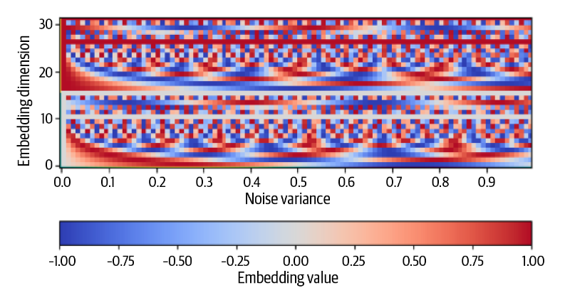
正弦编码器 sinusoidal_embedding

使用正弦编码器进行编码

这是一种将标量值映射到连续高位空间的方法，其编码方式可以被表示为：

$$\gamma(x)=\left(\sin \left(2 \pi e^{0 f} x\right), \cdots, \sin \left(2 \pi e^{(L-1) f)} x\right), \cos \left(2 \pi e^{0 f} x\right), \cdots, \cos \left(2 \pi e^{(L-1) f} x\right)\right)$$

我们可以选择$L = 16，f = \frac{\ln (1000)}{L-1}$进行建模。由此可以产生一个如下的编码模式。

其横坐标是$x$，即噪音的方差。纵坐标是其维度数，当我们选择$L = 16$时，有总共32个维度。所有的值都被映射在$[0,1]$之间。

将使用tensorflow实现的代码简单的替换为torch，即可复现正弦编码器的代码。

def sinusoidal_embedding(x):
    frequencies = torch.exp(
        torch.linspace(
            torch.log(1.0),
            torch.log(1000.0),
            NOISE_EMBEDDING_SIZE // 2,
        )
    )
    angular_speeds = 2.0 * torch.pi * frequencies
    embeddings = torch.concat(
        [torch.sin(angular_speeds * x), torch.cos(angular_speeds * x)], axis=3
    )
    return embeddings

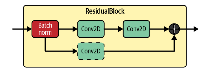
残差块 ResidualBlock

我们已经介绍过残差块，它可以帮助我们在更深的网络中学习更复杂的模式，避免梯度消失等原因带来的模型退化的影响。它的原理如图所示：

本程序中使用的残差块的跳跃连接并没有增加额外的卷积层，除非尺寸不契合。

在跳跃连接之外，模型包括一个批量归一化层和两个卷积层。它可以被简单的如下实现：

class ResidualBlock(nn.Module):
    def __init__(self,in_channels,out_channels):
        super(ResidualBlock,self).__init__()
        self.conv1 = nn.Conv2d(in_channels,out_channels,kernel_size=3,padding=1)
        self.conv2 = nn.Conv2d(out_channels,out_channels,kernel_size=3,padding=1)
        self.conv_residual = nn.Conv2d(in_channels,out_channels,kernel_size=1)
        self.bn = nn.BatchNorm2d(out_channels,affine=False)
        self.width = out_channels

    def forward(self,x):
        input_width = x.shape[1]
        if input_width == self.width:
            residual = x
        else:
            residual = self.conv_residual(x)
        x = self.bn(x)
        x = F.silu(self.conv1(x))
        x = self.conv2(x)
        x = x+residual
        return x

在实现中有两点需要注意的是：

• PyTorch在定义卷积层时需要输入通道数的参数。
• 在输入通道数不等于输出通道数时需要经过一个卷积核尺寸为1的卷积层来改变通道数。
• PyTorch的通道数是shape[1]而不是shape[3]

下采样和上采样块 DownBlock and UpBlock

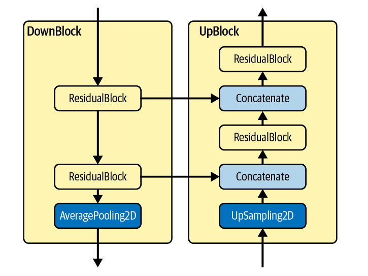
每个 DownBlock 都会通过ResidualBlocks增加通道数，同时还应用最终的AveragePooling2D 层，以便将图像的大小减半。每个 ResidualBlock 输出都会添加到列表中，供 UpBlock 层稍后使用。

class DownBlock(nn.Module):
    def __init__(self, in_channels,out_channels, block_depth):
        super(DownBlock, self).__init__()
        self.residual1 = ResidualBlock(in_channels, out_channels)
        self.residuals = nn.ModuleList([ResidualBlock(out_channels, out_channels) for _ in range(block_depth-1)])
        self.pool = nn.AvgPool2d(kernel_size=2)

    def forward(self, x):
        x, skips = x
        x = self.residual1(x)
        skips.append(x)
        for block in self.residuals:
            x = block(x)
            skips.append(x)
        x = self.pool(x)
        return x, skips

class UpBlock(nn.Module):
    def __init__(self, in_channels, out_channels, skips_channels, block_depth):
        super(UpBlock, self).__init__()
        self.residual1 = ResidualBlock(in_channels+skips_channels, out_channels)
        self.residuals = nn.ModuleList([ResidualBlock(out_channels+skips_channels, out_channels) for _ in range(block_depth-1)])
        self.up = nn.Upsample(scale_factor=2, mode='bilinear', align_corners=True)

    def forward(self, x):
        x, skips = x
        x = self.up(x)
        x = torch.cat([x, skips.pop()], dim=1)
        x = self.residual1(x)
        for block in self.residuals:
            x = torch.cat([x, skips.pop()], dim=1)
            x = block(x)
        return x, skips

在残差层的帮助下，我们可以很简单的定义这两个块。需要注意的是：

• 我们使用python风格的列表skips来实现两个块之间的信息共享，这个列表作为输入x的一部分，输入这两个块；然后以返回值输出，尽管这不是必要的。
• 只有第一个残差块的输入和输出维度不同，我们需要单独定义它们。
• UpBlock中引入了一个额外的参数skips_channels，指的是skips.pop()的维度，用于计算残差层的真实输入维度。这同样是因为PyTorch需要输入输入的尺寸而引入的。

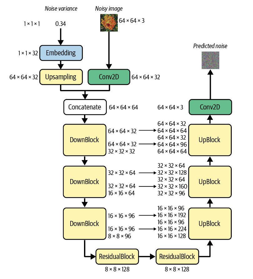
U-Net

在完成这些块的定义之后，我们定义最终的U-Net模型。

回顾我们在之前的部分给出过的结构图

这个模型包括两个输入：

• Noise Variance
• Noisy image

前者经过编码和上采样，后者者经过一个卷积层，变为相同的尺寸。连接后经过三个DownBlock，两个ResidualBlock，三个UpBlock，最后经过一个卷积层得到最终的预测噪音。

class UNet(nn.Module):
    def __init__(self, image_size):
        super(UNet, self).__init__()
        self.image_size = image_size
        # Noisy Image经过的第一个卷积层
        self.conv1 = nn.Conv2d(3, 32, kernel_size=1)
        # Noise variance 经过的两个层
        self.embedding = sinusoidal_embedding
        self.upsample = nn.Upsample(size=self.image_size, mode='nearest')
        # 三个DownBlock
        self.down1 = DownBlock(64, 32, block_depth=2)
        self.down2 = DownBlock(32, 64, block_depth=2)
        self.down3 = DownBlock(64, 96, block_depth=2)
        # 两个ResidualBlock
        self.res1 = ResidualBlock(96, 128)
        self.res2 = ResidualBlock(128, 128)
        # 三个UpBlock
        self.up1 = UpBlock(128, 96, 96, block_depth=2)
        self.up2 = UpBlock(96, 64, 64, block_depth=2)
        self.up3 = UpBlock(64, 32, 32, block_depth=2)
        # 最后一个卷积层
        self.conv2 = nn.Conv2d(32, 3, kernel_size=1)

我们根据上图中提到的每一层的信息，在__init__中定义这些层。

def forward(self, noisy_images, noise_variances):
     x = self.conv1(noisy_images)
     noise_embedding = self.embedding(noise_variances)
     noise_embedding = F.interpolate(noise_embedding)
     x = torch.cat([x, noise_embedding], dim=1)
     skips = []
     x, skips = self.down1([x,skips])
     x, skips = self.down2([x,skips])
     x, skips = self.down3([x,skips])
     x = self.res1(x)
     x = self.res2(x)
     x, skips = self.up1([x,skips])
     x, skips = self.up2([x,skips])
     x, skips = self.up3([x,skips])
     x = self.conv2(x)
     return x

得到完整的模型。

训练模型

接下来补充模型的训练过程

这里值得注意的是，扩散模型实际上维护了网络的两个副本：

• 使用梯度下降主动训练的
• EMA 网络：先前训练步骤中的权重的指数移动平均值。

EMA 网络不太容易受到训练过程中的短期波动和峰值的影响，这使得它比主动训练的网络更具有鲁棒性。因此，每当我们想要从网络生成生成的输出时，我们都会使用 EMA 网络。

了解训练过程

训练过程如下，仅仅看训练过程的话并不复杂。这些过程被定义在class DiffusionModel() 中。

def train_step(self,dataloader):
        self.network.train()
        self.ema_network.train()
        self.normalizer.adapt(dataloader)

        for epoch in range(EPOCHS):
            for i, (images, _) in enumerate(dataloader):
                images = self.normalizer(images.to(device))
                noises = torch.randn_like(images).to(device)
                # 获得扩散次数
                diffusion_times = torch.rand((BATCH_SIZE,1,1,1)).to(device)
                # 获得噪音率和信号率
                noise_rates, signal_rates = self.diffusion_schedule(diffusion_times)
                # 获得加入噪音后的图像
                noisy_images = images + noises * noise_rates
                # 获得去噪后的噪声和图像
                pred_noises, pred_images = self.denoise(noisy_images, noise_rates, signal_rates, training=True)
                
                # 计算损失
                noise_loss = self.loss(pred_noises, noises)
                # 反向传播
                self.optimizer.zero_grad()
                noise_loss.backward()
                self.optimizer.step()
                
                # 更新EMA网络
                for param, ema_param in zip(self.network.parameters(), self.ema_network.parameters()):
                    ema_param.data.mul_(EMA).add_((1 - EMA) * param.data)
                    
                print(f"Epoch {epoch}, Batch {i}, loss: {noise_loss.item()}")
            if epoch % 10 == 0:
                self.generate_print_image(10,PLOT_DIFFUSION_STEPS)

        return noise_loss

Normalizer层

self.normalizer 在PyTorch中并没有提供定义，按照tensorflow的文档的描述，可以近似实现这一层：

class normalizer(nn.Module):
    def __init__(self):
        super(normalizer, self).__init__()
        self.mean = torch.zeros(BATCH_SIZE, 3, 1, 1).to(device)
        self.std = torch.ones(BATCH_SIZE, 3, 1, 1).to(device)

    def adapt(self,dataloader):
        mean = []
        std = []
        for i, (images, _) in enumerate(dataloader):
            images = images.to(device)
            mean.append( torch.mean(images, dim=[0, 2, 3], keepdim=True).to(device))
            std.append( torch.std(images, dim=[0, 2, 3], keepdim=True).to(device))
        self.mean = torch.mean(torch.cat(mean, dim=0), dim=0, keepdim=True).expand(BATCH_SIZE,-1,-1,-1)
        self.std = torch.mean(torch.cat(std, dim=0), dim=0, keepdim=True).expand(BATCH_SIZE,-1,-1,-1)

    def forward(self, x):
        return (x - self.mean) / (self.std + 1e-8)

这个定义可以近似实现tensorflow的normalizer层的效果，但还存在一些差异。

结果分析

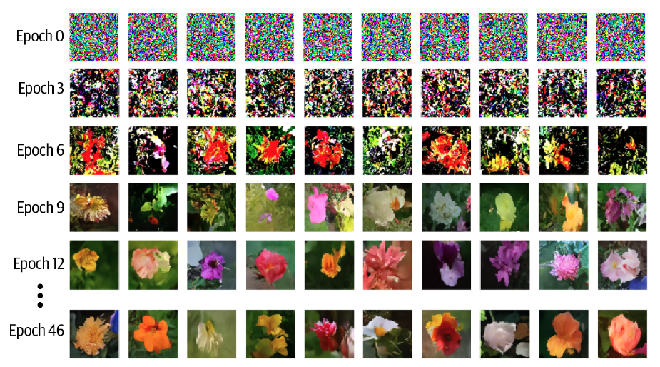
原书给出了类似这样的训练结果，可见最终的图像已经比较清晰。

💡 但我使用PyTorch实现的程序不能达到这样的效果。具体原因尚未排查出。目前看来有两个主要问题： - 其一是在epoch数比较低的时候学习的很慢，不能像上图所示在epoch = 6时就给出可以分辨的图像； - 其二是在epoch数比较高时会给出纯黑的图像。 目前在训练过程中观察到的问题可能包括loss在一定epoch后就不再有明显下降。 未来有时间应该逐步排查以下问题： - 数据是否被正确加载 - 尝试将输入图像归一化后反归一化，已验证归一化层知否正确实现 - 黑色图像是如何产生的 - 代码是否存在错误的实现 如果在实现本身没有问题，那问题可能出在超参数上的不匹配，或者PyTorch和Tensorflow对于一些函数实现上的差异。

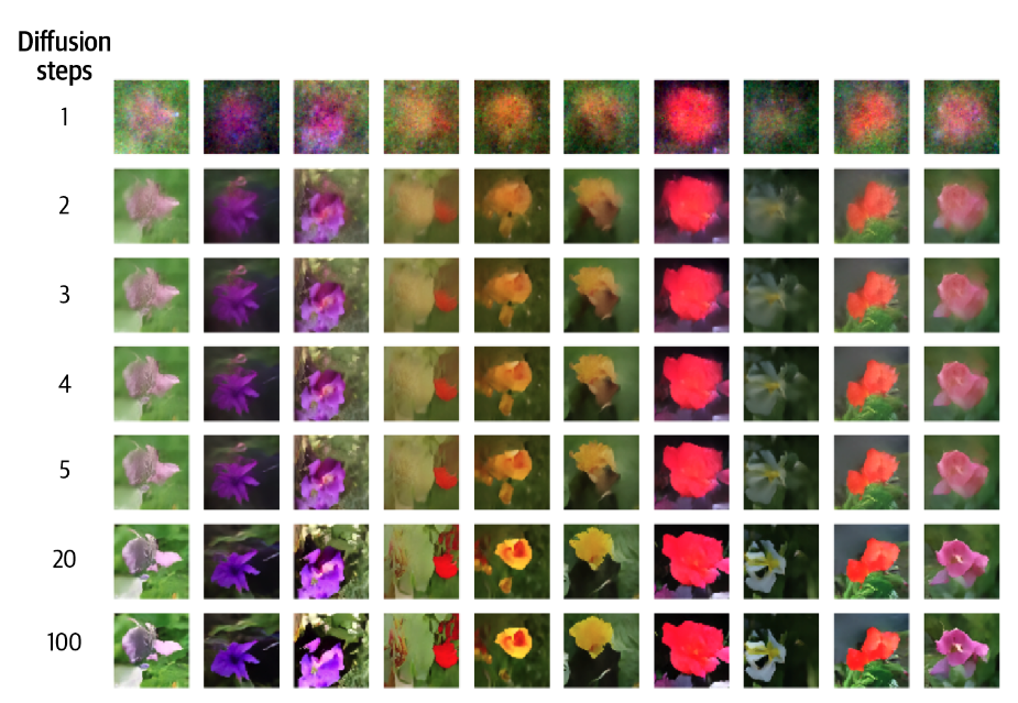
调整扩散步数

可以尝试在生成图像时使用不同的扩散步数，从下图的结果可以观察到，大约20步之后的步骤增加对图像质量影响不大。

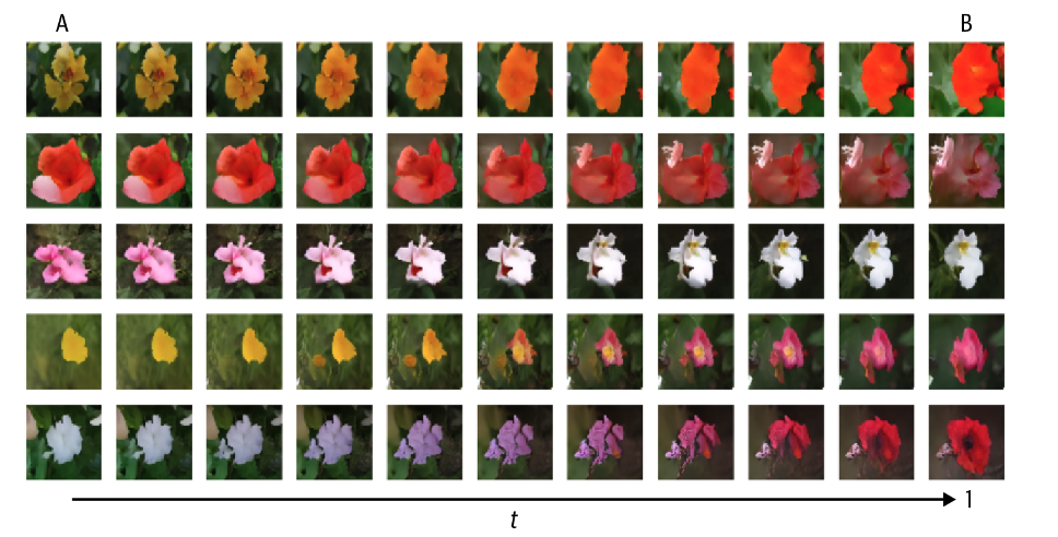
图像间的插值

与VAE类似，也可以使用插值的方式使生成的花朵在图像间过度。